What Are Two Key Differences Between BigQuery and Redshift?
Dec 15, 2021
Big Data. We often hear about this word but we aren’t quite sure how to define it. Literature says that having more than 1 TB of data can be considered as Big Data. After getting a mild idea of the concept, our next question would be: How can we manage such a large amount of data to find useful insights out of it? Well, one approach that can answer this lies in data warehousing.
A data warehouse is a data management system for storing and analyzing historical data. It enables business intelligence (BI) to perform queries and analysis on data. From renewable energy (General Electric) and clothing industry (American Eagle) to long-distance carpooling platforms (BlaBlaCar), enterprises rely on data warehouses to help them understand their customers’ experience by analyzing their logs over time.
In this article, we’ll compare the architecture and price of two of the major data warehouses currently leading the data market: AWS Redshift and BigQuery. Let’s get started!
Why Is Columnar Data Storage Important for Data Warehouses?
Accountants often use spreadsheets to report and keep track of their clients’ financial statements. By sequentially filling out data in rows, accountants can store from thousands to millions of financial entries. As this information grows, it can take up a lot of disk storage, and most importantly, when accountants perform any analysis on this data, reading each entry row-by-row ends up in a very time-consuming task.
Data warehouses, on the other hand, store data more efficiently in columns rather than in rows. The columnar data storage allows them to keep data closer together reducing seek time. A columnar design is also advantageous for preparing data for further distribution on several processing units. Data warehouses split up data and processing power among multiple compute resources that execute and coordinate operations simultaneously and in parallel, a process called massive parallel processing (MPP).
The row and columnar data design introduce two data processing capabilities: online transaction processing (OLTP) and online analytical processing (OLAP). OLTP transactions typically involve most or all of the columns in a row. Examples of this type are banking and ATM transactions that store data as a single record in a row. On the other hand, OLAP transactions read only a few columns from a very large number of rows. As you will see in the following section, this is the type of transactions that are involved with data warehouses.
Using Redshift or BigQuery, Does It Matter?
Now that you have a quick refresher of the fundamental concepts about data warehouses, let’s compare Redshift and BigQuery, which are two popular columnar storage-oriented data warehouses. In this section, we’ll help you decide which one to go with in terms of their architectural design and cost.
How Does Redshift Architecture Differ From That of BigQuery?
Let’s review the architectural styles of both data warehouses.
Redshift
AWS Redshift is a managed warehousing solution that is based on PostgreSQL. This is why it can be considered as a Relational Database Management System (RDBMS) compatible with most SQL clients applications and powerful enough to handle OLTP operations over rows. However, Redshift infrastructure goes far beyond because it is designed and optimized to manage Big Data workloads. In Redshift, you can create tables but their storage format will be slightly different from that of PostgreSQL. This is because Redshift stores data in a columnar format that improves query efficiency and speed.
The core of Redshift are clusters. A cluster is a collection of compute nodes. When a cluster includes two or more compute nodes, Redshift leverages a third node, known as the leader node, to orchestrate the incoming workload, see Figure 1. This node is the main point of contact between the client application and the compute nodes. The main responsibilities of the leader node are:
- Elaborate and execution plan
- Distribute data and workloads across compute nodes
- Gather results from compute nodes
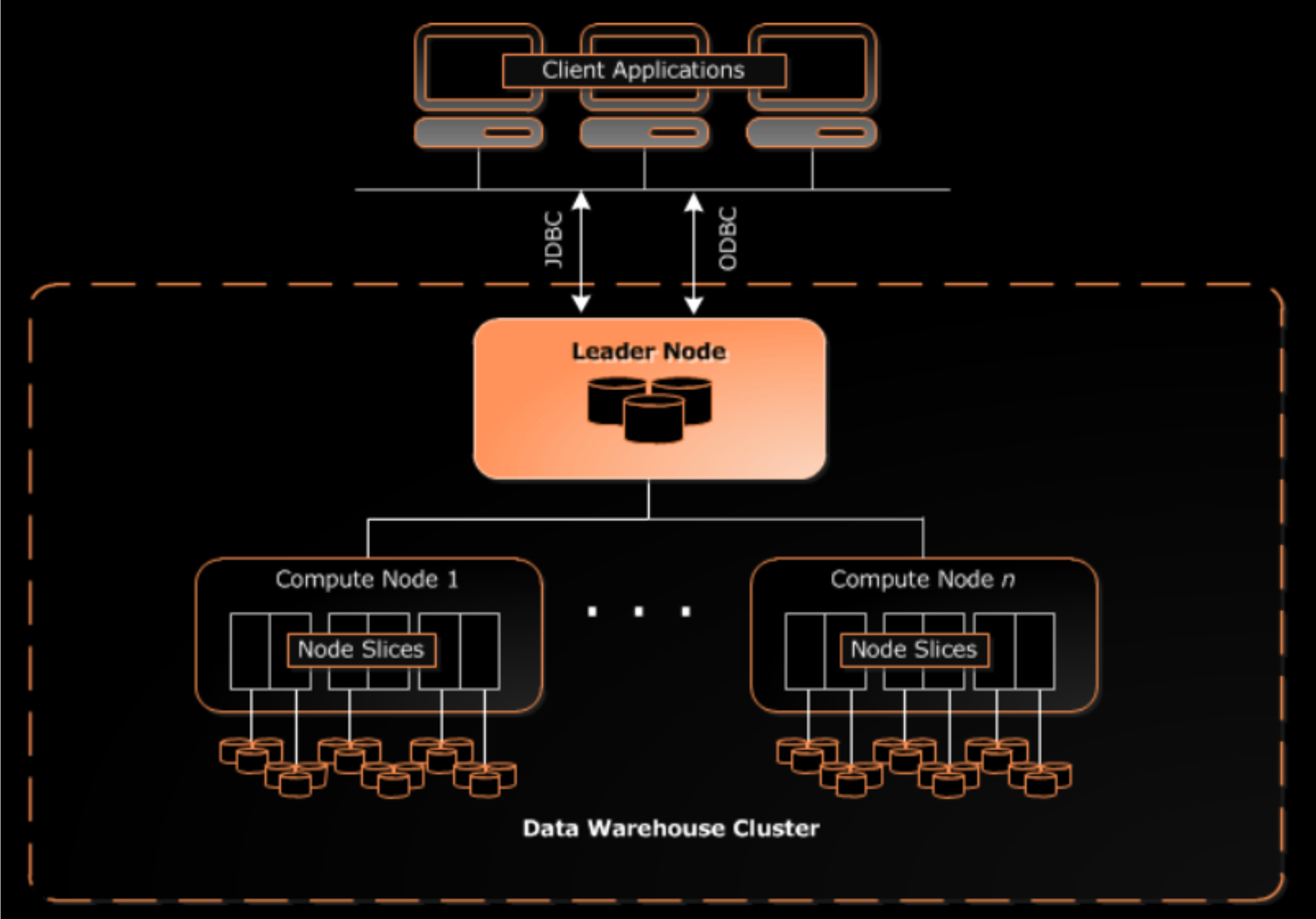 Figure 1. AWS Redshift architecture. Reference from AWS resources.
The capacity of a Redshift cluster is determined by the number of compute nodes and the node type. Each compute node has its own compute resources such as CPU, memory, and attached storage. The compute nodes redistribute compute resources across node slices and thus each node slice can have a compute power of a single CPU. All communications across nodes are handled through an internal AWS network.
Likewise resources, Redshift apportions user data in tables following a styling distribution scheme. Besides, you can select a column in a table that decides upon the sorting order of your data by using a sort key. This practice leverages data throughput and efficiency.
The interaction between AWS Redshift components resembles a Poker game played in teams. The dealer (lead node) is the point of contact between the cassino owner and the customers. Let’s say that the dealer sorts and distributes a deck of five cards across three teams, each one is led by a team leader (compute node) and composed by three members (node slices). Then, the team leader can redistribute the five cards among their teammates based on the card’s suit, color, or number (distribution style). When it is time to expose and compare hands to determine a winner, the leaders gather all cards (aggregates) from their teams and give them back to the dealer. Finally, the dealer notifies the house who is the winner.
BigQuery
BigQuery is a serverless data warehouse solution. Serverless means that you don’t need to worry about provisioning your infrastructure, BigQuery takes care of allocating resources on your behalf. Interestingly, its architecture decouples compute from storage, which means that you first have to bring your data, of any size, and then analyze it using standard SQL syntax. Under the hood, BigQuery employs low-level Google technologies such as Dremel, Borg, Colossus, and Jupiter to operate, as Figure 2 shows.
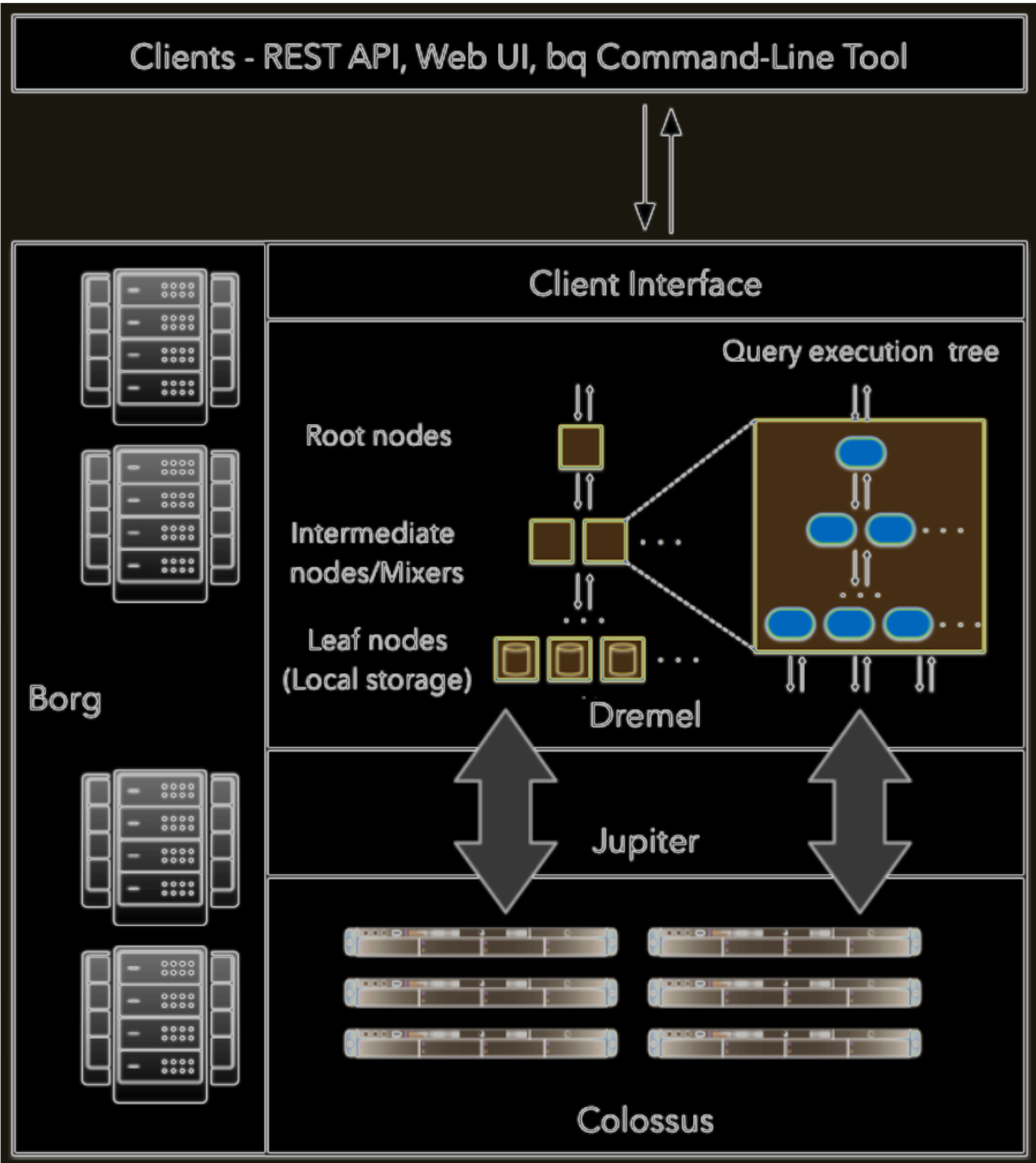 Figure 2. High-level architecture of BigQuery. Reference from Panoply
Let’s provide a summary of each technology:
Dremel. It handles computations and executes SQL queries. Depending on your query size and complexity, Dremel automatically calculates how many slots are required. A slot is a virtual CPU that represents the fundamental compute element of BigQuery. Dremel dynamically distributes queries from the client application to slots following an execution plan that resembles a tree structure. As Figure 2 shows, the execution plan starts on a root server (trunk) that apportions the workload across mixer nodes (branches). Mixers, in turn, redistribute the workload among leaf nodes (leaves), and so on.
Borg. It is an orchestrator that provisions root servers, mixer nodes, leaf nodes, and slots with hardware resources.
Colossus. It is the global storage system. Colossus servers store data in a columnar storage format and use a compression algorithm for handling Big Data optimally. Colossus’ primary tasks include fetching data to leaf nodes and handling data replication and recovery.
Jupyter. It is a Petabit network that establishes communication between compute and storage resources.
To understand BigQuery’s architecture, we can use a restaurant metaphor. You as the customer (client application) order a meal from the menu. The waiter (root server) takes your order to the chef (mixer). The chef then apportions your order across three groups of cooks (leaf nodes). Each group is responsible for preparing a specific component of your dish: salad, soup, and red meat. To start, the cooks need to gather all the ingredients from a big fridge (global storage system) located in another section of the kitchen. When each portion of your order is ready, the chef gathers each element, validates its flavour and quality, and turns it into a nice looking dish (aggregates). The chef passes on your meal to the waiter. Finally, the waiter serves the dish on your table. Bon appetit!
Answer
How does Redshift architecture differ from that of BigQuery? Primarily, Redshift is a node-based solution and BigQuery is a serverless solution. This translates into ease of use for the end-user. The following table shows the main architectural differences for both data warehouses:
| Redshift | BigQuery |
| It’s a node-based data warehouse | It's a serverless data warehouse solution |
| Couples compute and storage resources | Decouples compute and storage resources |
| Follows a top-down node hierarchy to execute queries | Follows a top-down slot hierarchy to execute queries |
| Requires to define beforehand the node type and number of nodes for your cluster unless you turn on concurrency scaling (might incur extra charges) | Scales up slots automatically based on on-demand workloads |
Is Redshift More Expensive Than BigQuery?
Let’s look at how the different architectures affect the cost of both solutions.
Redshift
As you can see in the previous section, AWS Redshift is a node-based data warehouse. Therefore, if you want to estimate the cost of your cluster, you need to determine beforehand the number of nodes and node types that your job will require. Determining the node size of your cluster is beyond the scope of this article, but you can find more information in About clusters and nodes. Let’s discuss about the three node types that AWS Redshift has:
- Dense Computing (DC2). Let’s consider the scenario where your data requires thousands of joins and aggregations of some of your results. Noticeably, these operations will consume a lot of compute resources. DC2 nodes are optimized to handle this type of compute-intense operations by providing compute resources with attached SSD storage. If your workload is not meant to grow, consider this node type as your best choice, otherwise you’ll need to add more nodes manually in order to store your results.
- Dense Storage (DS2). With this node you can create data warehouses that sit on hard disk drives (HDDs) resources. AWS recommends the usage of RA3 instead of DS2 nodes because of their better performance and cost.
- RA3. Perhaps you prefer an infrastructure that allows you to choose the number of nodes that you require and handle for you your storage resources. RA3 nodes fit into this category by implementing a managed storage solution that is independent from the compute resources. It takes away the burden of using DC2 nodes. RA3 nodes are optimal for BigData applications that require a storage solution that might scale up. In the event that the capacity of the SSD drive attached to the node is exceeded, RA3 nodes can scale their storage capacity by mananing offloads to S3 buckets without extra charges for using AWS S3.
The following table shows the cheapest node that you can spin up from each node type category. Extracted from AWS.
| Node Type | vCPU | Memory | Addressable storage capacity | I/O | Price |
| Dense Compute DC2 | |||||
| dc2.large | 2 | 15 GiB | 0.16TB SSD | 0.60 GB/s | $0.25 per Hour |
| Dense Storage DS2 | |||||
| ds2.xlarge | 4 | 31 GiB | 2TB HDD | 0.40 GB/s | $0.85 per Hour |
| RA3 with Redshift Managed Storage | |||||
| ra3.xlplus | 4 | 32 GiB | 32TB RMS | 0.65 GB/s | $1.086 per Hour |
Once you have chosen the node type and number of nodes for your cluster, you can take the most out of AWS pricing models:
- On-demand pricing model. Use this payment scheme under the basis of paying for what you use. There are no strings attached. Once you are done processing your data workload, you just simply turn off your cluster to avoid extra costs. This principing model is hourly rated, it follows the list of prices per node type described in the table above. So, the cheapest node you can run will cost you $0.25 per hour.
- Reserved Instances pricing model. If you consistently plan ahead your workloads, let’s say you run a job on a timely-basis, you can reserve nodes for one or three years. With this payment model, you can save up to 75% on on-demand prices ($0.0625 per hour for the cheapest node) when choosing for example an upfront payment option. If you have a limited initial budget, you can also explore other alternatives such as no upfront and partial upfront payment schemes.
- Spot instances pricing model. In case that you have spiky workloads runned at no particular schedule, you can consider this pricing model for your cluster. Let’s say that you need to extract, transform and load a batch of your data into an S3 bucket by the end of the day. This job takes you around 10 to 15 min. For this type of operation, AWS can offer you spare infrastructure for a short timeframe saving up-to 90% on on-demand prices ($0.025 per hour for the cheapest node). However, you should keep in mind that AWS can claim back these resources at any time.
BigQuery
BigQuery adds one layer of complexity to its pricing model because it splits up compute from storage resources. If you want to estimate your bill, keep in mind the following components of BigQuery pricing:
- Analysis. It is the cost of running queries, scripts, or functions. BigQuery offers two schemes: on-demand and flat-rate pricing. The on-demand scheme allows you to pay for the number of bytes processed by each query at a cost of $5 per TB. The amount of data processed by queries includes all selected data per column. Under this scheme, the slots units are not dedicated, which means that BigQuery can share this infrastructure with other clusters. If, on the other hand, you want to provision your cluster with dedicated infrastructure, the flat-rate pricing is your best choice. This is a region-oriented pricing scheme where you commit to the use of resources for a specific period of time:
- Per second. You pay for the use of 100 slots for $2920 per month. The commitment duration is only 60 seconds. You can cancel anytime once your commitment purchase is successful. Keep in mind that slots availability is not guaranteed.
- Per month. You pay for the use of 100 slots for $2000 per month.
- **Per year. **You pay for the use of 100 slots for $1700 per month.
- Storage. It is the cost of storing your data. BigQuery offers two schemes: active and long-term storage. The difference between both schemes relies upon the storage time frame. If you modify a table or partition of a table in the last 90 days (active storage), BigQuery charges you $0.02 per GB. In case that you exceed 90 consecutive days without doing any modification on your tables (long-term storage), BigQuery offers you a 50% discount on the active storage. For more details check Data size calculation.
- Extras. It includes costs related to data ingestion and extraction.
Answer
Is Redshift more expensive than BigQuery? Well, It depends on your use case. Here are the main takeaways about costs for both data warehouses:
| Redshift | BigQuery |
| Costs depend on the node type and number of nodes per cluster | It has two main pricing components: analysis and storage |
| Node types include DC2, DS2, and RA3 nodes. | Storage component comprises active and long-term storage pricing. You pay $0.02 per GB for modified tables in the last 90 days. |
| Nodes have hourly rates. The cheapest DC2 node you can spin up will cost you $0.25/h. | Analysis component comprises on-demand and flat-rate pricing. You pay $5 per TB for the number of bytes processed by each query |
| You can find great deals by reserving instances using upfront, no upfront, and partial upfront pricing schemes. | You can find great deals by committing to the use of resources for a specific period of time: per second, per month, and per year. |
So, Which Data Warehouse Is Better To Use?
We don’t have in fact an actual winner out of this comparison article. Both Redshift and BigQuery are data warehouses that have gained their status as leading products in the current data market. However, through our analysis of their architectural style and cost, we have identified differences that can help you decide when to choose a data warehouse solution based on your needs.
In our opinion, Redshift’s architecture provides greater flexibility to end-users to fine-tune resources according to their needs, which can impact on performance and cost. However, Redshift end-users should have an intermediate technical knowledge base to provision compute nodes by choosing the correct node type and the right number of nodes. In terms of cost, Redshift establishes hourly rates per cluster, which is quite cost-effective for programmed workloads like ETLs.
On the other hand, BigQuery’s serverless solution brings simplicity. Provisioning of resources is on BigQuery’s behalf, which can benefit entry-level end-users who only need to upload their data and start creating SQL queries. Because BigQuery decouples storage and compute, estimating costs based on its pricing model is rather complex. However, we believe that BigQuery is optimal for spiky workloads because it charges you per processed data instead of having to pay a full hour.
We encourage you to take a step further this fundamental understanding of both data warehouses. Create a free account and get hands-on experience with AWS and GCP free tier.